Confidence interval for a mean • interpretCI

This document is prepared automatically using the following R command.

Problem

Confidence interval of mean

The approach that we used to solve this problem is valid when the following conditions are met.

The sampling method must be simple random sampling.
The sampling distribution should be approximately normally distributed.

Since the above requirements are satisfied, we can use the following four-step approach to construct a confidence interval of mean.

Raw data

The first 10 rows of the provided data is as follows.

 [38;5;246m# A tibble: 10 × 1 [39m
     mpg
    [3m [38;5;246m<dbl> [39m [23m
 [38;5;250m 1 [39m  21  
 [38;5;250m 2 [39m  21  
 [38;5;250m 3 [39m  22.8
 [38;5;250m 4 [39m  21.4
 [38;5;250m 5 [39m  18.7
 [38;5;250m 6 [39m  18.1
 [38;5;250m 7 [39m  14.3
 [38;5;250m 8 [39m  24.4
 [38;5;250m 9 [39m  22.8
 [38;5;250m10 [39m  19.2

Sample statistics

The sample size is 32, the sample mean is 20.09 and the standard error of sample is 6.03. The confidence level is 95 %.

Find the margin of error

Since we do not know the standard deviation of the population, we cannot compute the standard deviation of the sample mean; instead, we compute the standard error (SE). Because the sample size is much smaller than the population size, we can use the “approximate” formula for the standard error.

\[ SE= \frac{s}{\sqrt{n}}\] where s is the standard deviation of the sample, n is the sample size.

\[SE=\frac{6.03}{\sqrt{32}}=1.07\] Find the critical probability(p*):

\[p*=1-\alpha/2=1-0.05/2=0.975\]

The degree of freedom(df) is: \[df=n-1=32-1=31\]

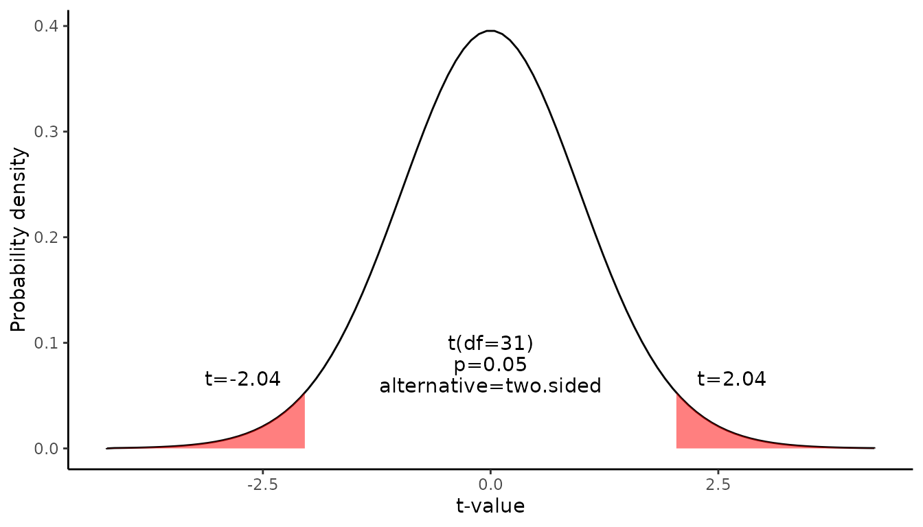
The critical value is the t statistic having 31 degrees of freedom and a cumulative probability equal to 0.975. From the t Distribution table, we find that the critical value is 2.04.

df	0.400	0.250	0.100	0.050	0.025	0.010	0.005	0.001
29	-0.256	-0.683	-1.311	-1.699	-2.045	-2.462	-2.756	-3.396
30	-0.256	-0.683	-1.310	-1.697	-2.042	-2.457	-2.750	-3.385
31	-0.256	-0.682	-1.309	-1.696	-2.040	-2.453	-2.744	-3.375
32	-0.255	-0.682	-1.309	-1.694	-2.037	-2.449	-2.738	-3.365

\[qt(p,df)=qt(0.975,31)=2.04\]

The graph shows the \(\alpha\) values are the tail areas of the distribution.

Compute margin of error(ME):

\[ME=critical\ value \times SE\] \[ME=2.04 \times 1.065=2.173\]

Specify the confidence interval. The range of the confidence interval is defined by the sample statistic \(\pm\)margin of error. And the uncertainty is denoted by the confidence level.

Confidence interval of the mean

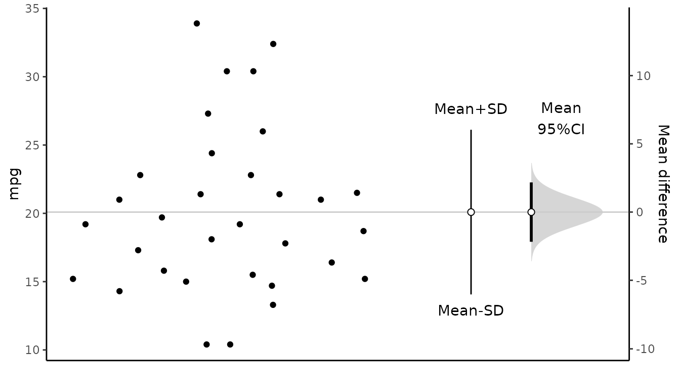
Therefore, the 95% confidence interval is 17.92 to 22.26. That is, we are 95% confident that the true population mean is in the range 17.92 to 22.26.

Plot

You can visualize the mean difference:

Result of meanCI()


call: meanCI.data.frame(x = mtcars, mpg) 
method: One sample t-test 
alternative hypothesis:
   true mean  is not equal to  0 

Results
 [38;5;246m# A tibble: 1 × 7 [39m
  m        se     DF    lower    upper    t      p        
   [3m [38;5;246m<chr> [39m [23m     [3m [38;5;246m<chr> [39m [23m   [3m [38;5;246m<chr> [39m [23m  [3m [38;5;246m<chr> [39m [23m     [3m [38;5;246m<chr> [39m [23m     [3m [38;5;246m<chr> [39m [23m   [3m [38;5;246m<chr> [39m [23m    
 [38;5;250m1 [39m 20.09062 1.0654 31    17.91768 22.26357 18.857 < 2.2e-16

Reference

The contents of this document are modified from StatTrek.com. Berman H.B., “AP Statistics Tutorial”, [online] Available at: https://stattrek.com/estimation/confidence-interval-mean.aspx?tutorial=AP URL[Accessed Data: 1/23/2022].