Hypothesis test for the difference between proportions

This document is prepared automatically using the following R command.

Problem

Solution

This lesson explains how to conduct a hypothesis test to determine whether the difference between two proportions is significant.

The test procedure, called the two-proportion z-test, is appropriate when the following conditions are met:

• The sampling method for each population is simple random sampling.

• The samples are independent.

• Each sample includes at least 10 successes and 10 failures.

• Each population is at least 20 times as big as its sample.

This approach consists of four steps: (1) state the hypotheses, (2) formulate an analysis plan, (3) analyze sample data, and (4) interpret results.

Since the above requirements are satisfied, we can use the following four-step approach to construct a confidence interval.

1. State the hypotheses

The first step is to state the null hypothesis and an alternative hypothesis.

\[Null\ hypothesis(H_0): P_1 \leqq P_2\] \[Alternative\ hypothesis(H_1): P_1 > P_2\]

Note that these hypotheses constitute a one-tailed test. The null hypothesis will be rejected if the proportion from population 1 is too big..

2. Formulate an analysis plan

For this analysis, the significance level is 0.05`. The test method, shown in the next section, is a two-proportion z-test.

3. Analyze sample data

Using sample data, we calculate the pooled sample proportion (p) and the standard error (SE). Using those measures, we compute the z-score test statistic (z).

\[p=\frac{p_1 \times n_1+ p_2 \times n_2}{n1+n2}\] \[p=\frac{0.71 \times 150+ 0.63 \times 100}{150+100}\]

\[p=169.5/250=0.678\]

\[SE=\sqrt{p\times(1-p)\times[1/n_1+1/n_2]}\]

\[SE=\sqrt{0.678\times0.322\times[1/150+1/100]}=0.061\]

\[z=\frac{p_1-p_2}{SE}=\frac{0.71-0.63}{0.061}=1.33\]

where \(p_1\) is the sample proportion in sample 1, where \(p_2\) is the sample proportion in sample 2, \(n_1\) is the size of sample 1, and \(n_2\) is the size of sample 2.

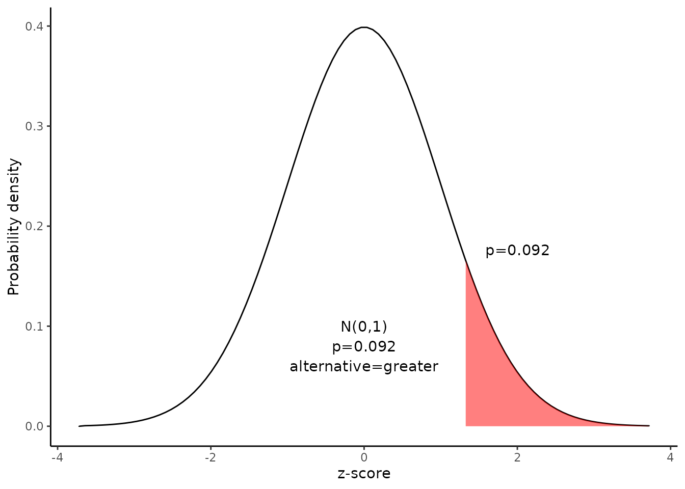
Since we have a one-tailed test, the P-value is the probability that the z statistic is or greater than 1.33.

We can use following R code to find the p value.

\[p=pnorm(1.33,lower.tail=FALSE)=0.092\]

Alternatively,we can use the Normal Distribution curve to find p value.

draw_n(z=x$result$z,alternative=x$result$alternative)

4. Interpret results.

Since the P-value (0.092) is greater than the significance level (0.05), we cannot reject the null hypothesis.

Result of propCI()

$data

[38;5;246m# A tibble: 1 × 2
[39m
  x     y    
  
[3m
[38;5;246m<lgl>
[39m
[23m 
[3m
[38;5;246m<lgl>
[39m
[23m

[38;5;250m1
[39m 
[31mNA
[39m    
[31mNA
[39m   

$result
  alpha   p1   p2  n1  n2  DF   pd         se critical        ME      lower
1  0.05 0.71 0.63 150 100 248 0.08 0.06085776 1.644854 0.1001021 -0.0201021
      upper                      CI ppooled   sepooled        z     pvalue
1 0.1801021 0.08 [95CI -0.02; 0.18]   0.678 0.06032081 1.326242 0.09237975
  alternative
1     greater

$call
propCI(n1 = 150, n2 = 100, p1 = 0.71, p2 = 0.63, P = 0, alternative = "greater")

attr(,"measure")
[1] "propdiff"

Reference

The contents of this document are modified from StatTrek.com. Berman H.B., “AP Statistics Tutorial”, [online] Available at: https://stattrek.com/hypothesis-test/difference-in-proportions.aspx?tutorial=AP URL[Accessed Data: 1/23/2022].