Confidence interval for the unpaired mean difference
Source:vignettes/Confidence_interval_for_unpaired_mean_difference.Rmd
Confidence_interval_for_unpaired_mean_difference.RmdThis document is prepared automatically using the following R command.
library(interpretCI) |
Problem
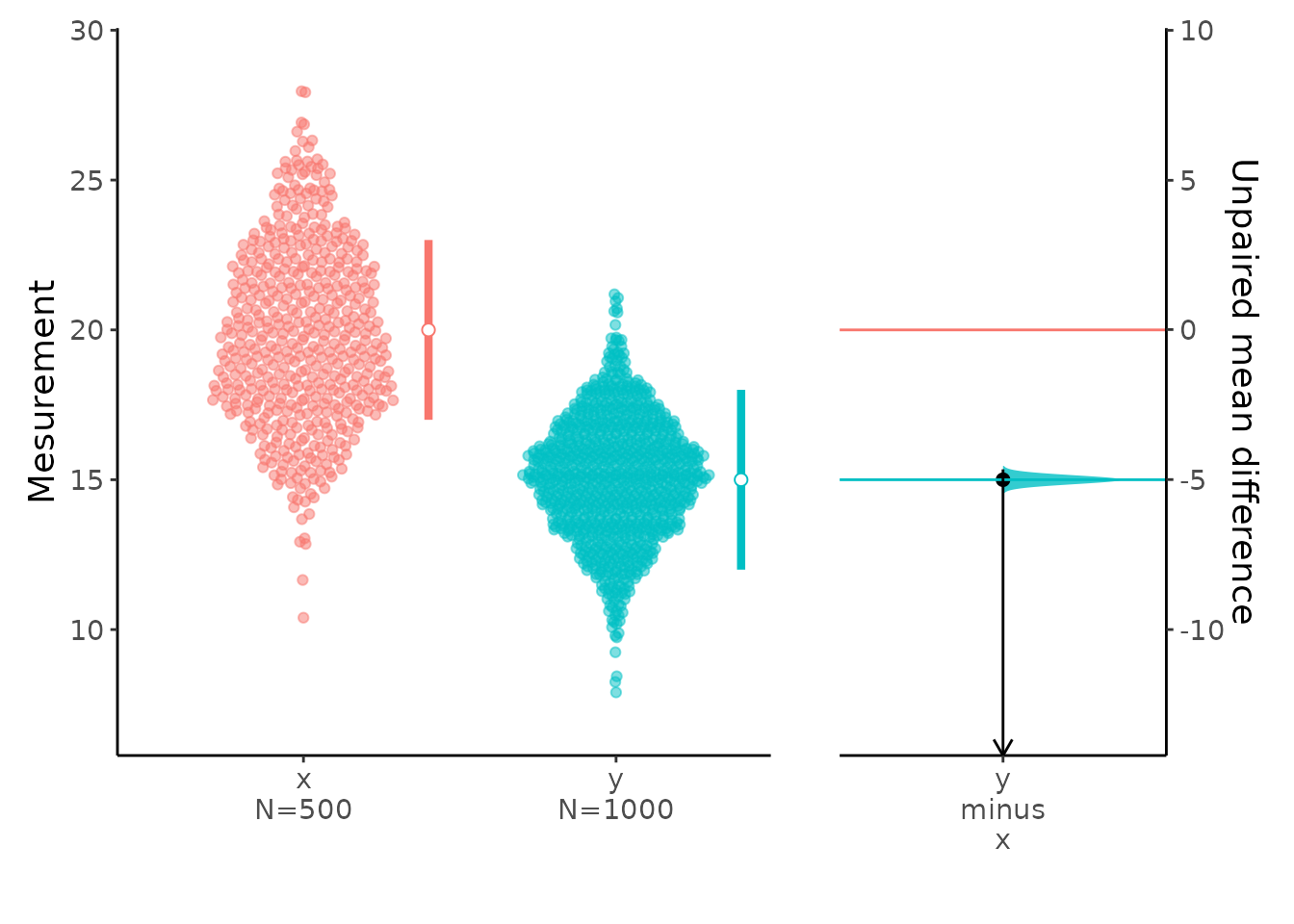
The local baseball team conducts a study to find the amount spent on refreshments at the ball park. Over the course of the season they gather simple random samples of 500 men and 1000 women. For men, the average expenditure was $ 20, with a standard deviation of $ 3. For women, it was $15, with a standard deviation of $2. |
Confidence interval of mean
The approach that we used to solve this problem is valid when the following conditions are met.
The sampling method must be simple random sampling.
The samples must be independent.
The sampling distribution should be approximately normally distributed.
Since the above requirements are satisfied, we can use the following four-step approach to construct a confidence interval of mean.
Identify sample statistics
Since we are trying to estimate the difference between population means, we choose the difference between sample means as the sample statistic. Thus,
\[\bar{x1}-\bar{x2}=20-15=5\]
Select a confidence level.
In this analysis, the confidence level is defined for us in the problem. We are working with a 99% confidence level.
Find the margin of error
1. Find standard error.
The standard error is an estimate of the standard deviation of the difference between population means. We use the sample standard deviations to estimate the standard error (SE).
\[SE=\sqrt{\frac{s^2_1}{n_1}+\frac{s^2_2}{n_2}}\] \[SE=\sqrt{\frac{3^2}{500}+\frac{2^2}{1000}}\] \[SE=0.148\]
2. Find the degree of freedom(df)
\[DF=\frac{(\frac{s_1^2}{n_1}+\frac{s_2^2}{n_2})^2}{\frac{(s_1^2/n_1)^2}{n_1-1}+\frac{(s_2^2/n_2)^2}{n_2-1}}\] \[DF=\frac{(\frac{3^2}{500}+\frac{2^2}{1000})^2}{\frac{(3^2/500)^2}{500-1}+\frac{(2^2/1000)^2}{1000-1}}\]
\[DF=727.48\]
3. Find the critical value
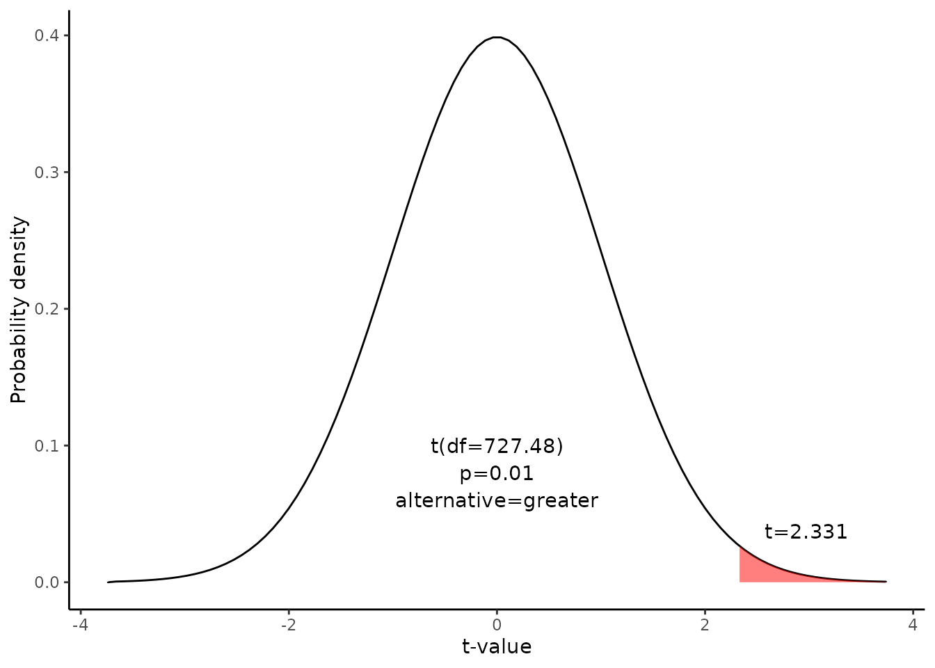
The critical value is the t statistic having 727.48 degrees of freedom and a cumulative probability equal to 0.99. From the t Distribution table, we find that the critical value is 2.331.
df |
0.400 |
0.250 |
0.100 |
0.050 |
0.025 |
0.010 |
0.005 |
0.001 |
725 |
-0.253 |
-0.675 |
-1.283 |
-1.647 |
-1.963 |
-2.332 |
-2.583 |
-3.102 |
726 |
-0.253 |
-0.675 |
-1.283 |
-1.647 |
-1.963 |
-2.331 |
-2.583 |
-3.101 |
727 |
-0.253 |
-0.675 |
-1.283 |
-1.647 |
-1.963 |
-2.331 |
-2.583 |
-3.101 |
728 |
-0.253 |
-0.675 |
-1.283 |
-1.647 |
-1.963 |
-2.331 |
-2.583 |
-3.101 |
\[ qt(p,df)=qt(0.99,727.48)=2.331\] The graph shows that \(\alpha\) values are the tail areas of the distribution.

Confidence interval of the mean difference
Therefore, the 99% confidence interval is 4.65 to Inf. Here’s how to interpret this confidence interval. Suppose we repeated this study with different random samples for men and women. Based on the confidence interval, we would expect the observed difference in sample means to be between 4.65 and Inf 99% of the time.
Result of meanCI()
call: meanCI.default(n1 = 500, n2 = 1000, m1 = 20, s1 = 3, m2 = 15,      s2 = 2, alpha = 0.01, alternative = "greater")
method: Welch Two Sample t-test
alternative hypothesis:
   true unpaired differences in means is greater than  0

Results

[38;5;246m# A tibble: 1 × 6
[39m
  control test  DF     CI                    t     p

[3m
[38;5;246m<chr>
[39m
[23m
[3m
[38;5;246m<chr>
[39m
[23m
[3m
[38;5;246m<chr>
[39m
[23m
[3m
[38;5;246m<chr>
[39m
[23m
[3m
[38;5;246m<chr>
[39m
[23m
[3m
[38;5;246m<chr>
[39m
[23m

[38;5;250m1
[39m x       y     727.48 5.00 [99CI 4.65; Inf] 33.71 < 2.2e-16
Reference
The contents of this document are modified from StatTrek.com. Berman H.B., “AP Statistics Tutorial”, [online] Available at: https://stattrek.com/estimation/difference-in-means.aspx?tutorial=AP URL[Accessed Data: 1/23/2022].
