Hypothesis test for a mean

This document is prepared automatically using the following R command.

Given Problem : Two-Tailed Test

This lesson explains how to conduct a hypothesis test of a mean, when the following conditions are met:

The sampling method is simple random sampling.
The sampling distribution is normal or nearly normal.

Generally, the sampling distribution will be approximately normally distributed if any of the following conditions apply.

The population distribution is normal.
The population distribution is symmetric, unimodal, without outliers, and the sample size is 15 or less.
The population distribution is moderately skewed, unimodal, without outliers, and the sample size is between 16 and 40.
The sample size is greater than 40, without outliers.

This approach consists of four steps:

state the hypotheses
formulate an analysis plan
analyze sample data
interpret results.

1. State the hypotheses

The first step is to state the null hypothesis and an alternative hypothesis.

\[Null\ hypothesis(H_0): \mu = 23\] \[Alternative\ hypothesis(H_1): \mu \neq 23\]

Note that these hypotheses constitute a two-tailed test. The null hypothesis will be rejected if the sample mean is too big or if it is too small..

2. Formulate an analysis plan

For this analysis, the significance level is 95%. The test method is a one-sample t-test.

3. Analyze sample data.

Using sample data, we compute the standard error (SE), degrees of freedom (DF), and the t statistic test statistic (t).

\[SE = \frac{s}{\sqrt{n}} = \frac{6.0269481}{\sqrt{32}} = 1.07\] \[DF=n-1=32-1=31\]

\[t = (\bar{x} - \mu) / SE = (20.090625 - 23)/1.07 = -2.731\]

where s is the standard deviation of the sample, \(\bar{x}\) is the sample mean, \(\mu\) is the hypothesized population mean, and n is the sample size.

We can visualize the confidence interval of mean.

plot(x)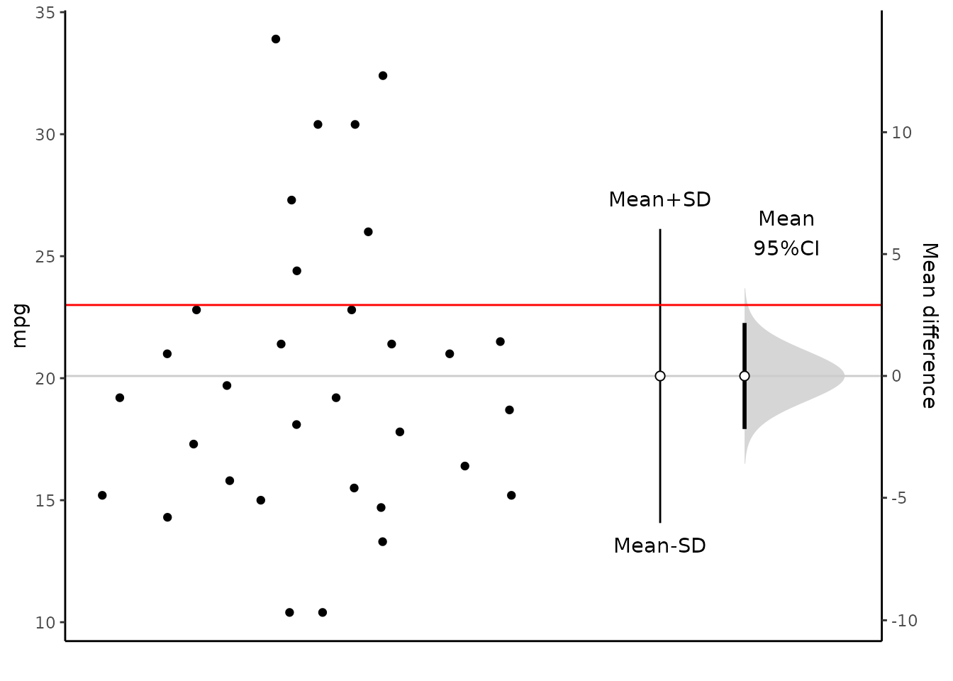

Since we have a two-tailed test, the P-value is the probability that the t statistic having 31 degrees of freedom is less than -2.73 or greater than 2.73.

We use the t Distribution curve to find p value.

draw_t(DF=x$result$DF,t=x$result$t,alternative=x$result$alternative)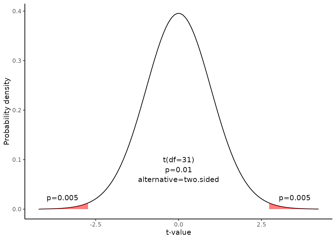

\[pt(-2.731,31) =0.01 \]

4. Interpret results.

Since the P-value (0.01) is less than the significance level (0.05), we can reject the null hypothesis.

Result of meanCI()


call: meanCI.data.frame(x = mtcars, mpg, mu = 23) 
method: One sample t-test 
alternative hypothesis:
   true mean  is not equal to  23 

Results
 [38;5;246m# A tibble: 1 × 7 [39m
  m        se     DF    lower    upper    t       p      
   [3m [38;5;246m<chr> [39m [23m     [3m [38;5;246m<chr> [39m [23m   [3m [38;5;246m<chr> [39m [23m  [3m [38;5;246m<chr> [39m [23m     [3m [38;5;246m<chr> [39m [23m     [3m [38;5;246m<chr> [39m [23m    [3m [38;5;246m<chr> [39m [23m  
 [38;5;250m1 [39m 20.09062 1.0654 31    17.91768 22.26357 -2.7307 0.01033

Reference

The contents of this document are modified from StatTrek.com. Berman H.B., “AP Statistics Tutorial”, [online] Available at: https://stattrek.com/hypothesis-test/mean.aspx?tutorial=AP URL[Accessed Data: 1/23/2022].