Hypothesis test for a proportion
Source:vignettes/Hypothesis_test_for_a_proportion.Rmd
Hypothesis_test_for_a_proportion.RmdThis document is prepared automatically using the following R command.
library(interpretCI) |
Problem
The CEO of a large electric utility claims that 20 percent of his 10000 customers are very satisfied with the service they receive. To test this claim, the local newspaper surveyed 100 customers, using simple random sampling. Among the sampled customers, 27 percent say they are very satisified. Based on these findings, can we reject the CEO's hypothesis that 20% of the customers are very satisfied? Use a 0.01 level of significance. |
Confidence interval of a sample proportion
The approach that we used to solve this problem is valid when the following conditions are met.
The sampling method must be simple random sampling. This condition is satisfied; the problem statement says that we used simple random sampling.
Each sample point can result in just two possible outcomes. We call one of these outcomes a success and the other, a failure.
The sample should include at least 10 successes and 10 failures. Suppose we classify a “more local news” response as a success, and any other response as a failure. Then, we have 0.73 \(\times\) 100 = 73 successes, and 0.27 \(\times\) 100 = 27 failures - plenty of successes and failures.
The population size is at least 20 times as big as the sample size. If the population size is much larger than the sample size, we can use an approximate formula for the standard deviation or the standard error. This condition is satisfied, so we will use one of the simpler approximate formulas.
This approach consists of four steps:
state the hypotheses
formulate an analysis plan
analyze sample data
interpret results.
1. State the hypotheses
The first step is to state the null hypothesis and an alternative hypothesis.
\[Null\ hypothesis(H_0): P = 0.8\] \[Alternative\ hypothesis(H_1): P \neq 0.8\]
Note that these hypotheses constitute a two-tailed test. The null hypothesis will be rejected if the sample proportion is too big or if it is too small..
2. Formulate an analysis plan
For this analysis, the significance level is 0.01`. The test method, shown in the next section, is a one-sample z-test.
2. Select a confidence level.
In this analysis, the confidence level is defined for us in the problem. We are working with a 99% confidence level.
3. Analyze sample data
Using sample data, we calculate the standard deviation (sd) and compute the z-score test statistic (z).
\[sd=\sqrt{\frac{P\times(1-P)}{n}}\] \[sd=\sqrt{\frac{0.8\times(1-0.8)}{100}}=0.04\] \[z=\frac{p-P}{sd}=\frac{0.73-0.8}{0.04}=-1.75\] where \(P\) is the hypothesized value of population proportion in the null hypothesis, \(p\) is the sample proportion, and \(n\) is the sample size.
Since we have a two-tailed test, the P-value is the probability that the z statistic is less than -1.75 or greater than 1.75.
We can use following R code to find the p value.
\[p=pnorm(-abs(-1.75))\times2=0.08\]
Alternatively,we can use the Normal Distribution curve to find p value.
draw_n(z=x$result$z,alternative=x$result$alternative)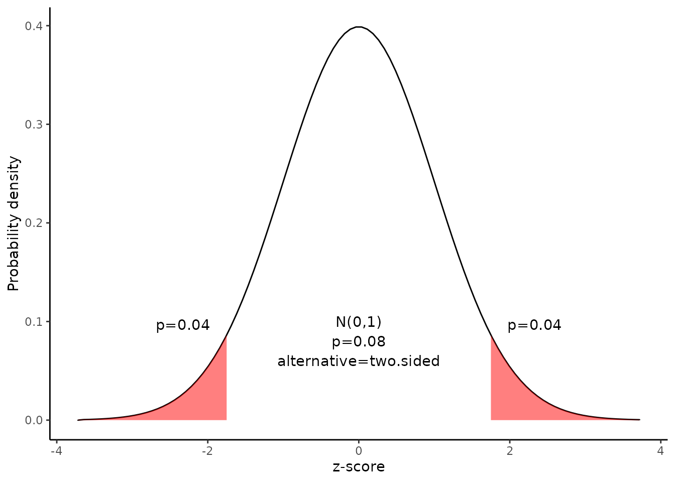
4. Interpret results.
Since the P-value (0.08) is greater than the significance level (0.01), we cannot reject the null hypothesis.
Result of propCI()
$data

[38;5;246m# A tibble: 1 × 1
[39m
  value

[3m
[38;5;246m<lgl>
[39m
[23m

[38;5;250m1
[39m
[31mNA
[39m

$result
  alpha   n df    p   P   se critical        ME     lower     upper
1  0.01 100 99 0.73 0.8 0.04 2.575829 0.1030332 0.6269668 0.8330332
                      CI     z     pvalue alternative
1 0.73 [99CI 0.63; 0.83] -1.75 0.08011831   two.sided

$call
propCI(n = 100, p = 0.73, P = 0.8, alpha = 0.01)

attr(,"measure")
[1] "prop"
Reference
The contents of this document are modified from StatTrek.com. Berman H.B., “AP Statistics Tutorial”, [online] Available at: https://stattrek.com/hypothesis-test/proportion.aspx?tutorial=AP URL[Accessed Data: 1/23/2022].