S3 method for an object of class "meanCI"
Usage
# S3 method for meanCI
plot(x, ref = "control", side = NULL, palette = NULL, ...)
Arguments
- x
an object of class "meanCI"
- ref
string One of c("test","control").
- side
logical or NULL If true draw side by side plot
- palette
The name of color palette from RColorBrewer package or NULL
- ...
Further arguments to be passed
Value
A ggplot or an object of class "plotCI" containing at least the following components: '
- p1
A ggplot
- p2
A ggplot
- side
logical
Examples
meanCI(mtcars,mpg) %>% plot()
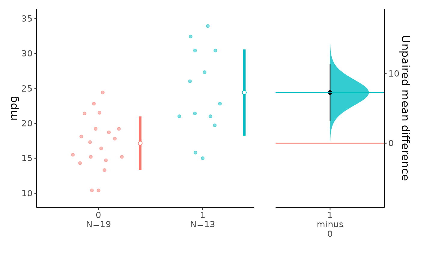
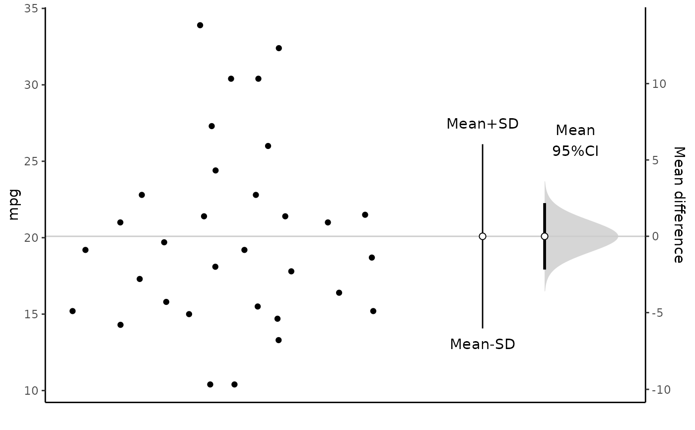 meanCI(mtcars,am,mpg) %>% plot()
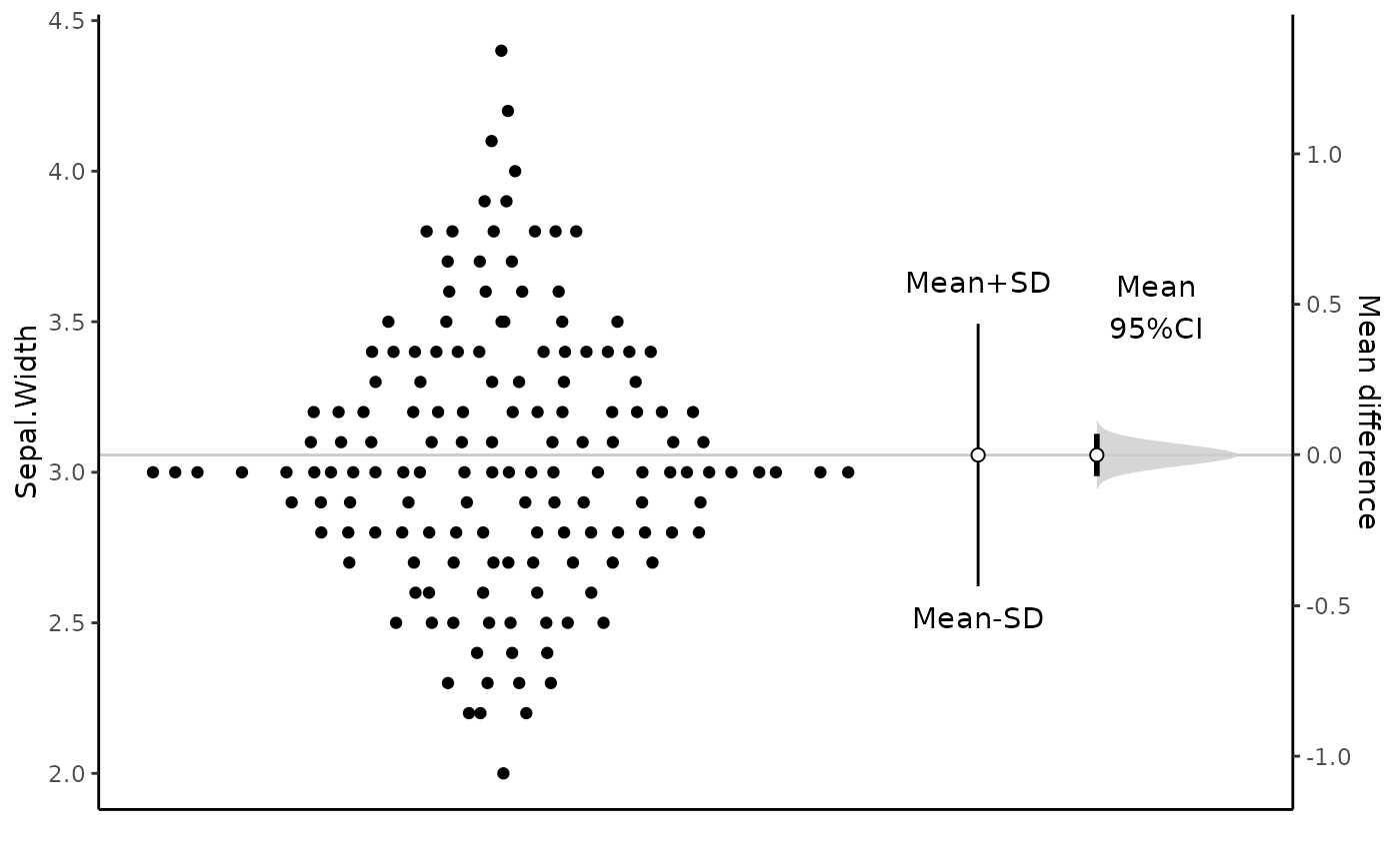
 meanCI(iris,Sepal.Width) %>% plot()
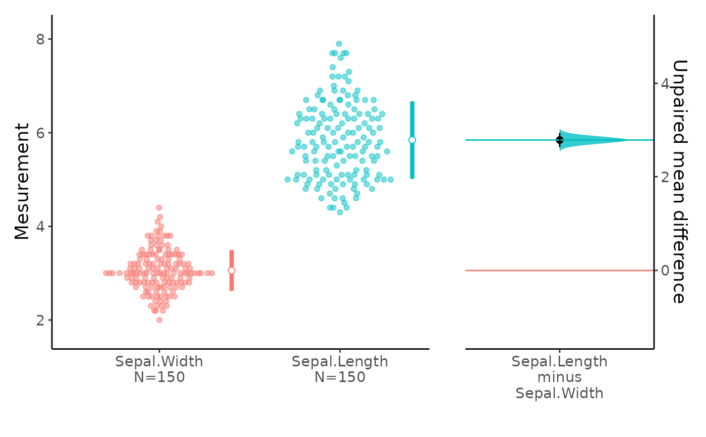
 meanCI(iris,Sepal.Width,Sepal.Length) %>% plot()
 # \donttest{
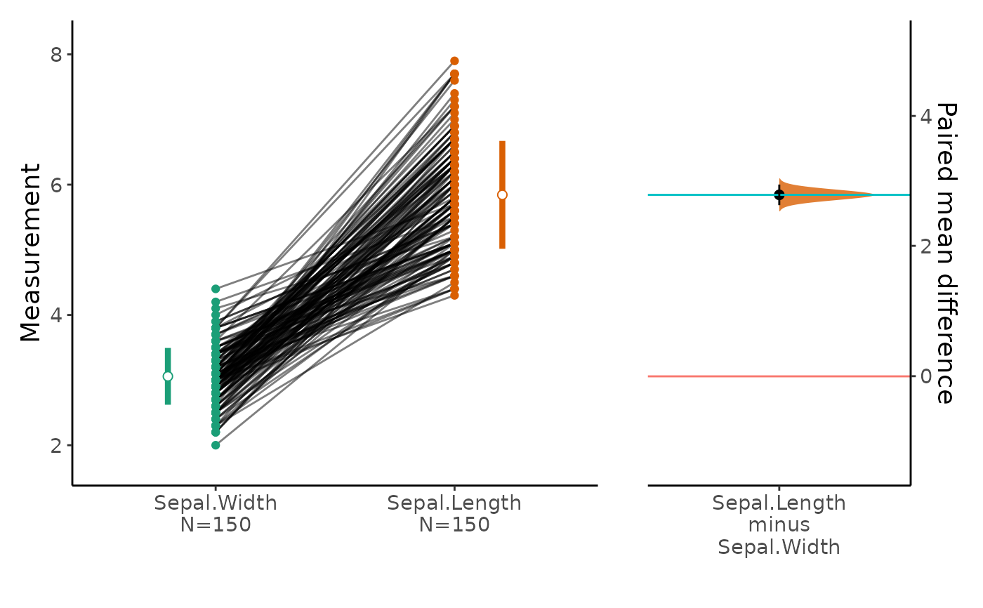
meanCI(iris,Sepal.Width,Sepal.Length,paired=TRUE) %>% plot(palette="Dark2")
# \donttest{
meanCI(iris,Sepal.Width,Sepal.Length,paired=TRUE) %>% plot(palette="Dark2")
 meanCI(iris,Sepal.Width,Sepal.Length) %>% plot()
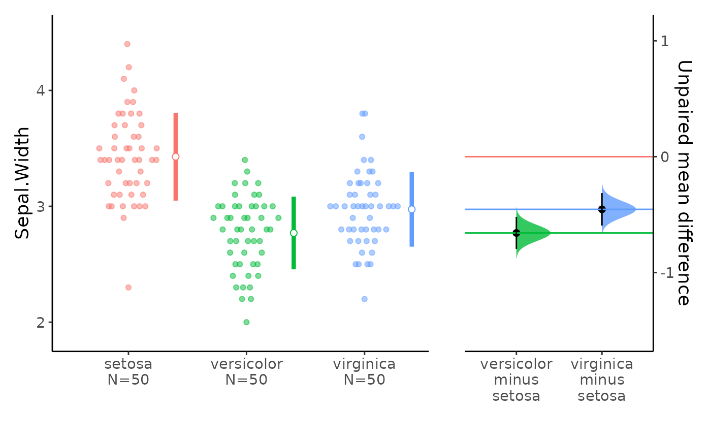
 meanCI(iris,Species,Sepal.Width) %>% plot(side=TRUE)
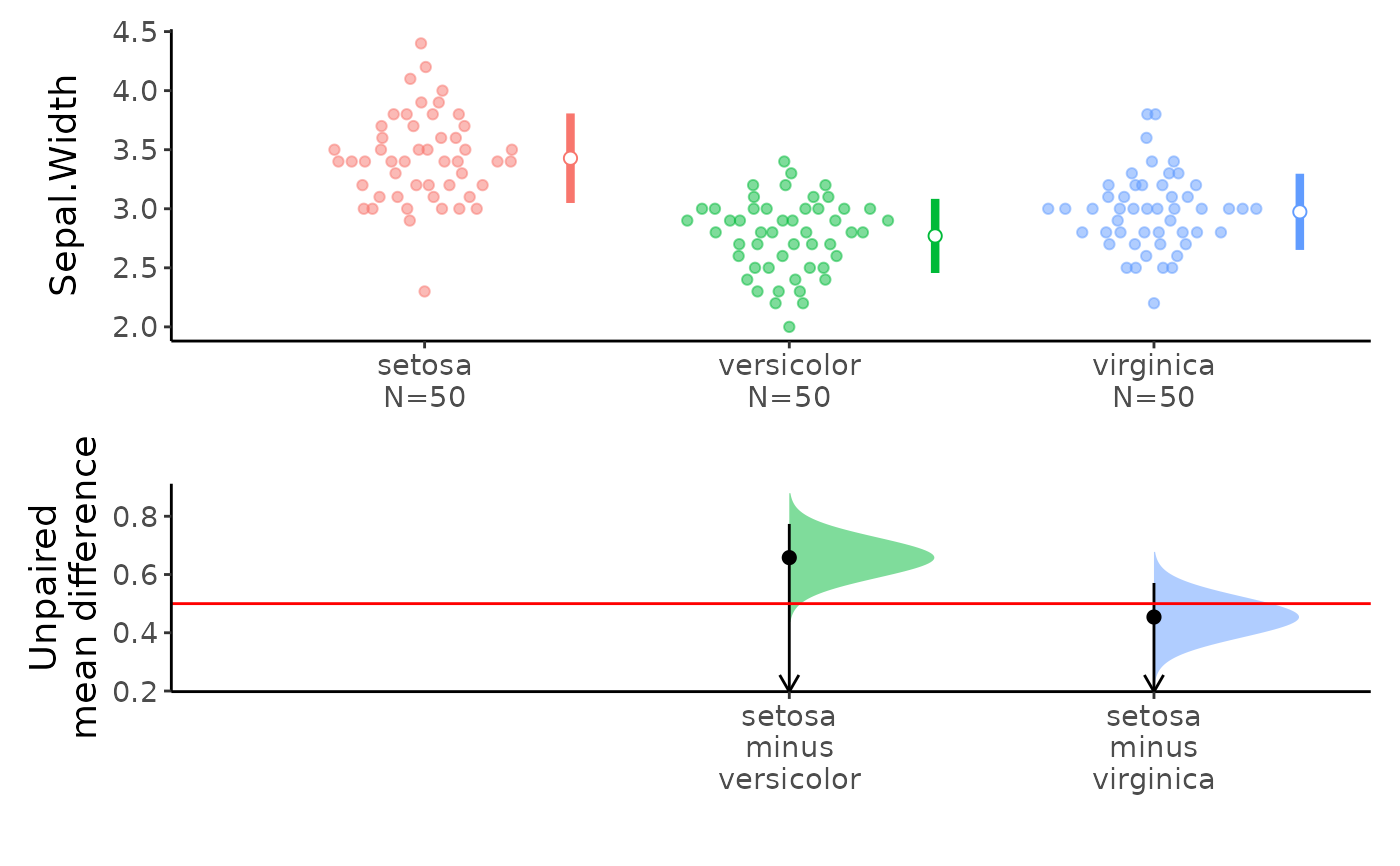
 meanCI(iris,Species,Sepal.Width,mu=0.5,alternative="less") %>% plot(ref="test")
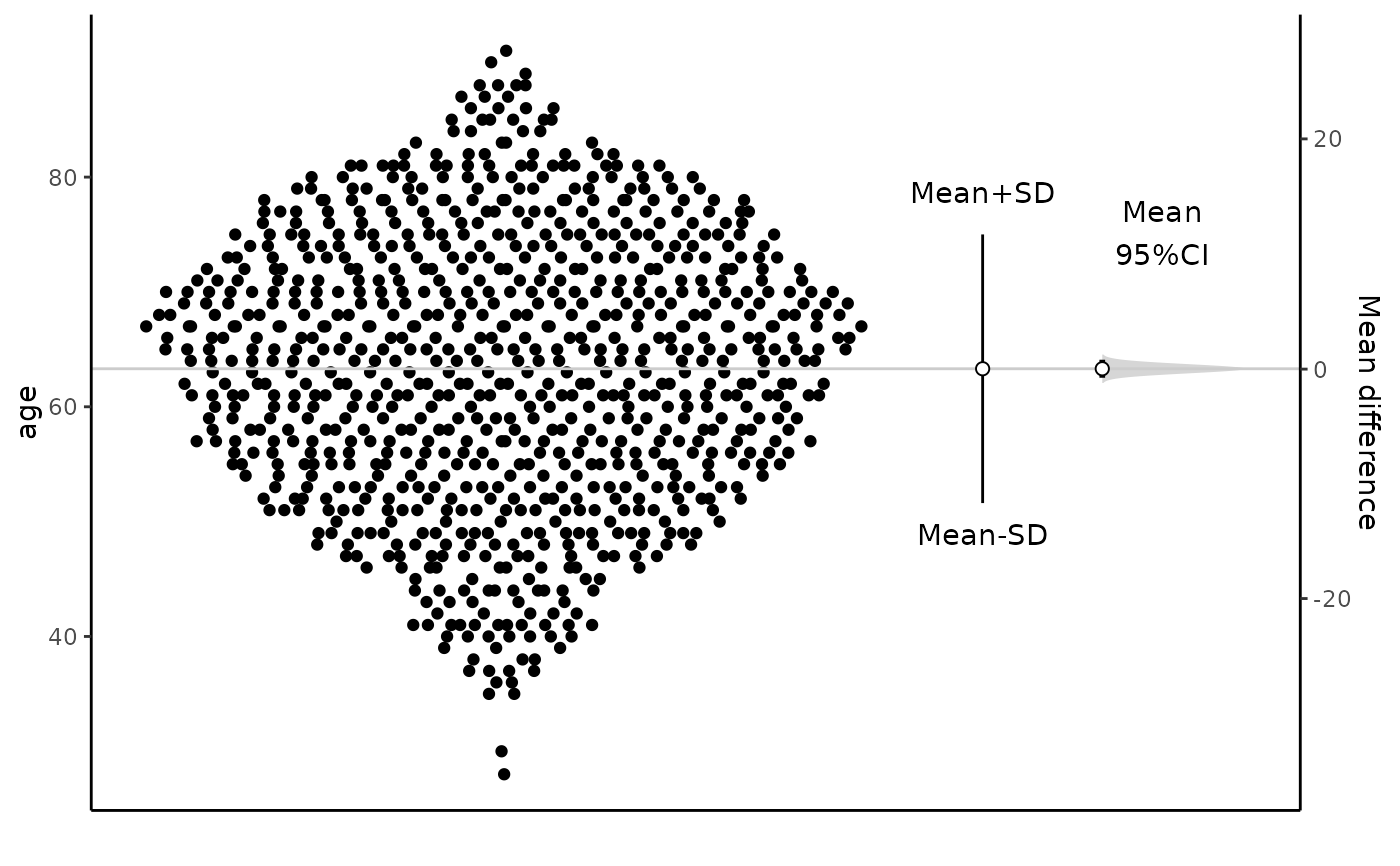
 meanCI(acs,age) %>% plot()
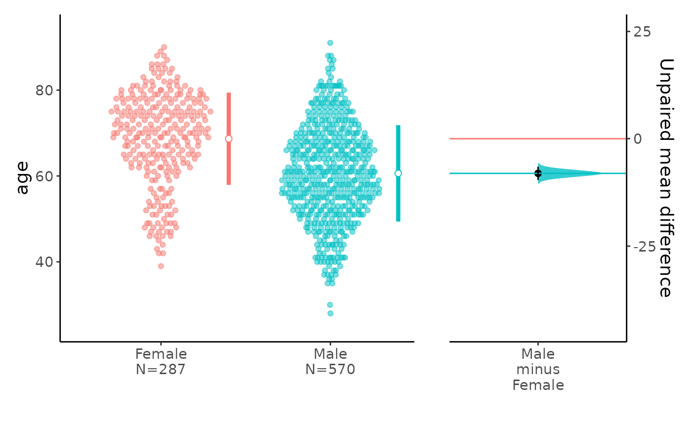
 meanCI(acs,sex,age) %>% plot()
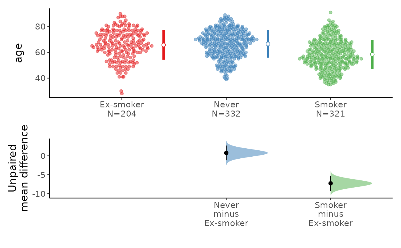
 meanCI(acs,smoking,age) %>% plot(palette="Set1")
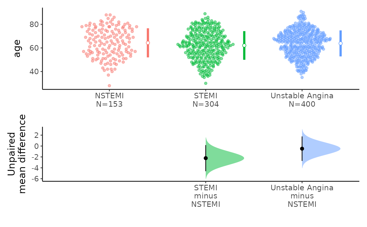
 meanCI(acs,Dx,age) %>% plot()
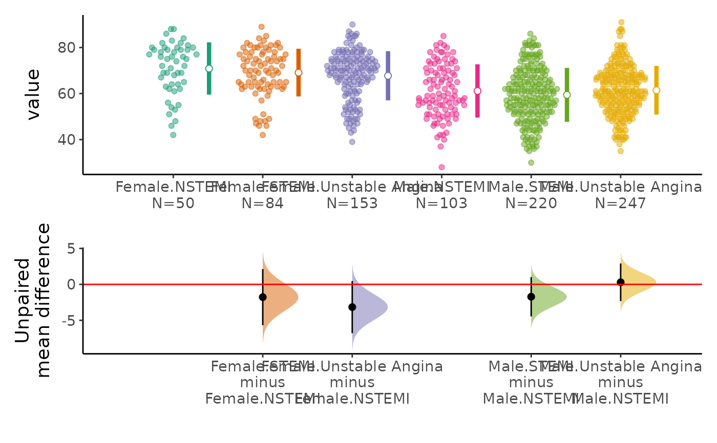
 meanCI(acs,Dx,age,sex,mu=0) %>% plot(palette="Dark2")
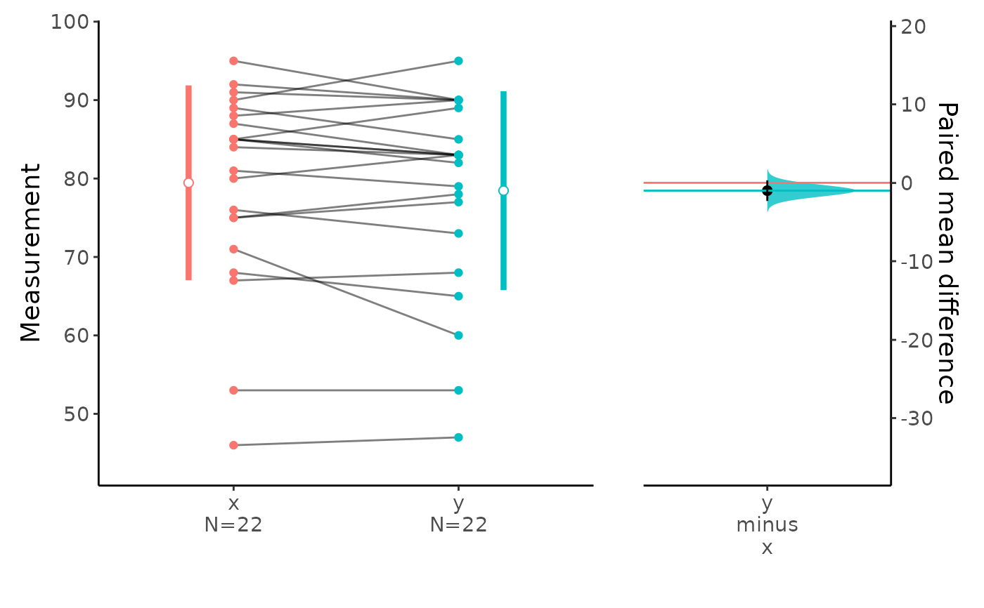
 x=c(95,89,76,92,91,53,67,88,75,85,90,85,87,85,85,68,81,84,71,46,75,80)
y=c(90,85,73,90,90,53,68,90,78,89,95,83,83,83,82,65,79,83,60,47,77,83)
meanCI(x=x,y=y,paired=TRUE,alpha=0.1) %>% plot()
x=c(95,89,76,92,91,53,67,88,75,85,90,85,87,85,85,68,81,84,71,46,75,80)
y=c(90,85,73,90,90,53,68,90,78,89,95,83,83,83,82,65,79,83,60,47,77,83)
meanCI(x=x,y=y,paired=TRUE,alpha=0.1) %>% plot()
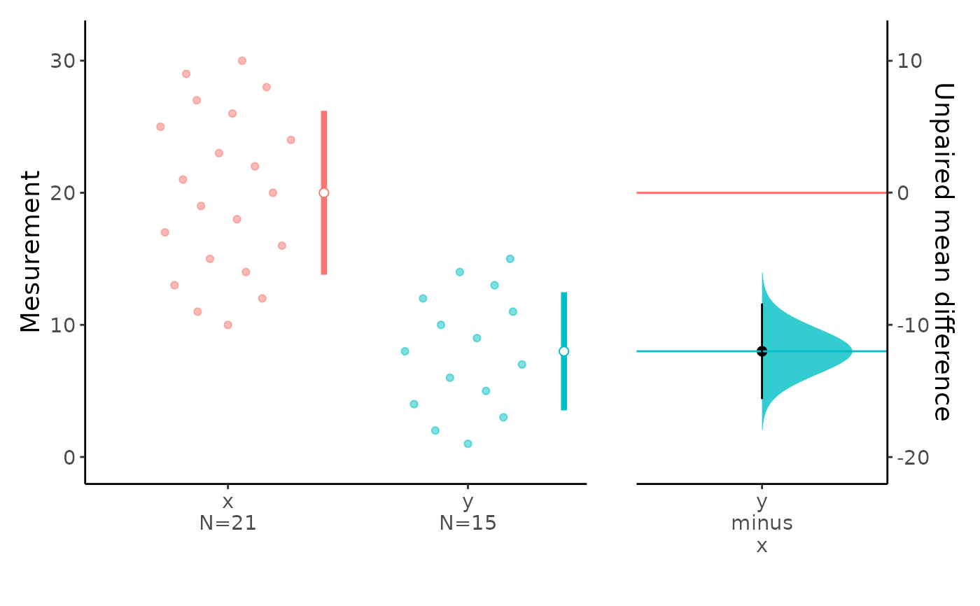
 meanCI(10:30,1:15) %>% plot()
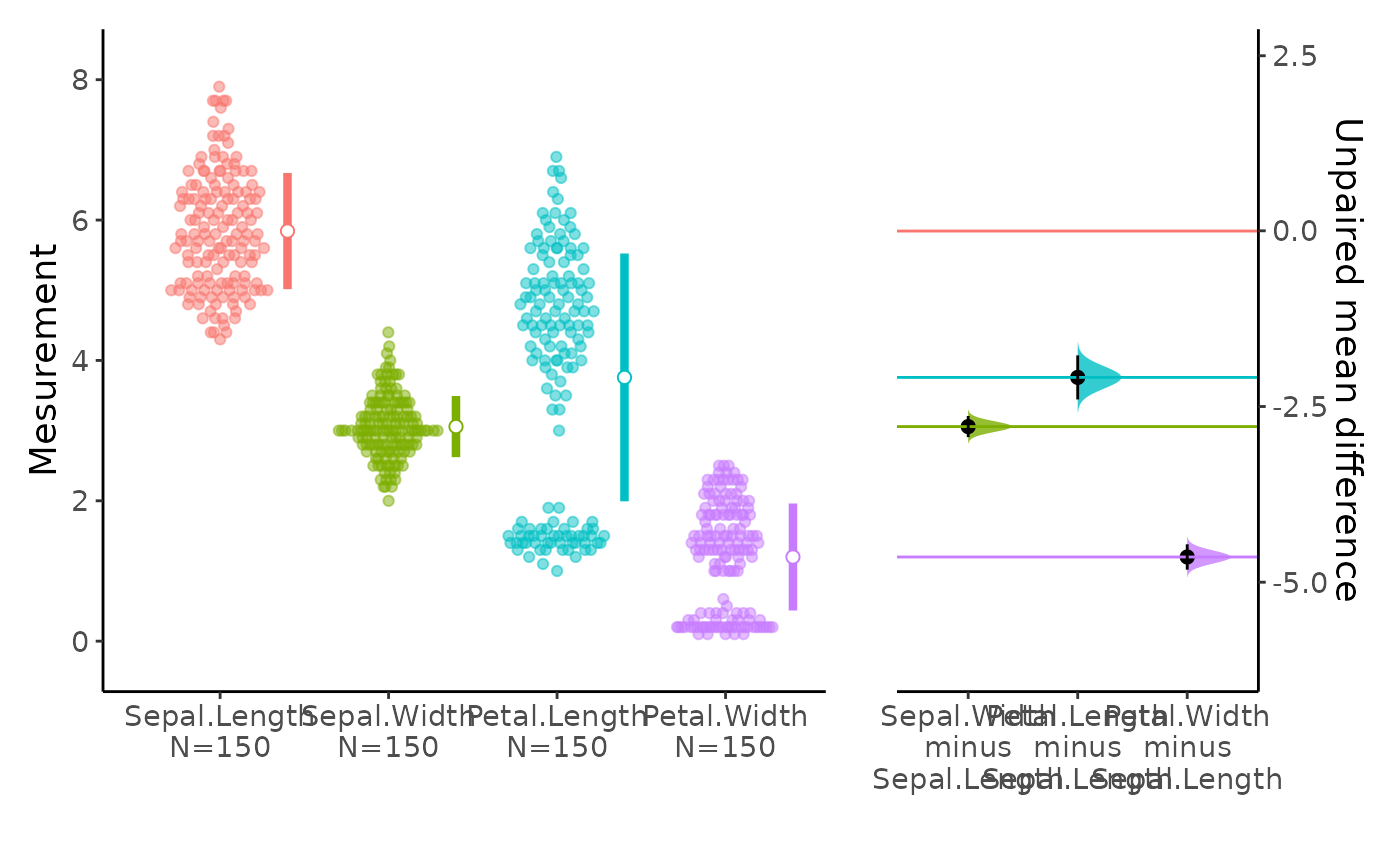
 iris %>% meanCI() %>% plot(side=TRUE)
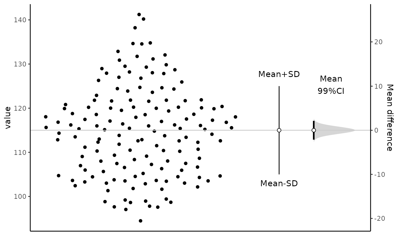
 meanCI(n=150,m=115,s=10,alpha=0.01) %>% plot()
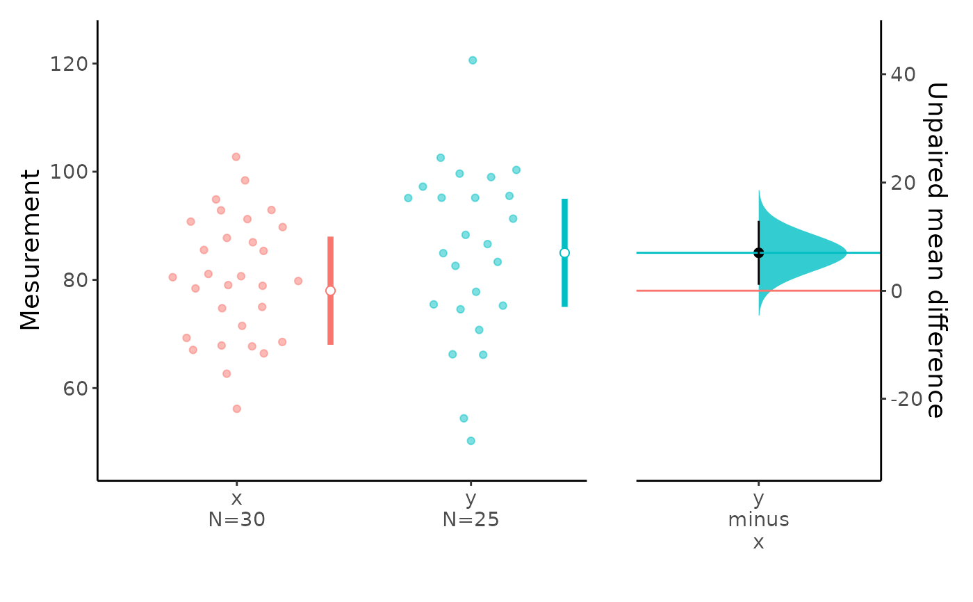
 meanCI(n1=30,n2=25,m1=78,s1=10,m2=85,s2=15,alpha=0.10) %>% plot()
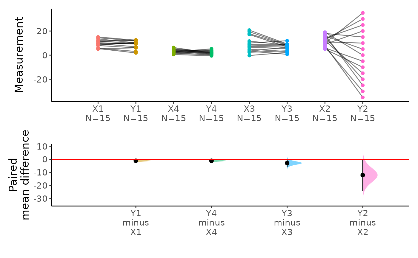
 data(anscombe2,package="PairedData")
meanCI(anscombe2,idx=list(c("X1","Y1"),c("X4","Y4"),c("X3","Y3"),c("X2","Y2")),
paired=TRUE,mu=0) %>% plot()
data(anscombe2,package="PairedData")
meanCI(anscombe2,idx=list(c("X1","Y1"),c("X4","Y4"),c("X3","Y3"),c("X2","Y2")),
paired=TRUE,mu=0) %>% plot()
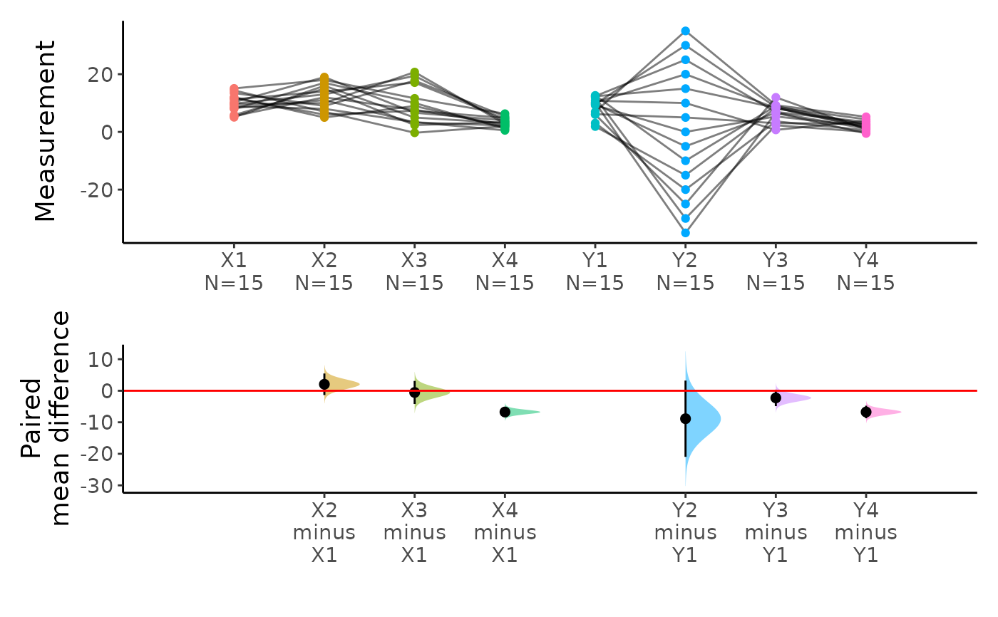
 x=meanCI(anscombe2,idx=list(c("X1","X2","X3","X4"),c("Y1","Y2","Y3","Y4")),paired=TRUE,mu=0)
plot(x)
x=meanCI(anscombe2,idx=list(c("X1","X2","X3","X4"),c("Y1","Y2","Y3","Y4")),paired=TRUE,mu=0)
plot(x)
 longdf=tidyr::pivot_longer(anscombe2,cols=X1:Y4)
x=meanCI(longdf,name,value,idx=list(c("X1","X2","X3","X4"),c("Y1","Y2","Y3","Y4")),paired=TRUE,mu=0)
plot(x)
longdf=tidyr::pivot_longer(anscombe2,cols=X1:Y4)
x=meanCI(longdf,name,value,idx=list(c("X1","X2","X3","X4"),c("Y1","Y2","Y3","Y4")),paired=TRUE,mu=0)
plot(x)
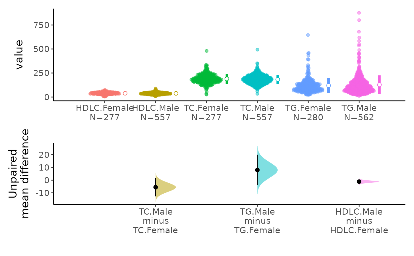
 acs %>% select(sex,TC,TG,HDLC) %>% meanCI(group=sex) %>% plot()
#> Warning: Removed 61 rows containing missing values (position_quasirandom).
#> Warning: Removed 61 rows containing missing values (position_quasirandom).
#> Warning: Removed 61 rows containing missing values (position_quasirandom).
#> Warning: Removed 61 rows containing missing values (position_quasirandom).
acs %>% select(sex,TC,TG,HDLC) %>% meanCI(group=sex) %>% plot()
#> Warning: Removed 61 rows containing missing values (position_quasirandom).
#> Warning: Removed 61 rows containing missing values (position_quasirandom).
#> Warning: Removed 61 rows containing missing values (position_quasirandom).
#> Warning: Removed 61 rows containing missing values (position_quasirandom).
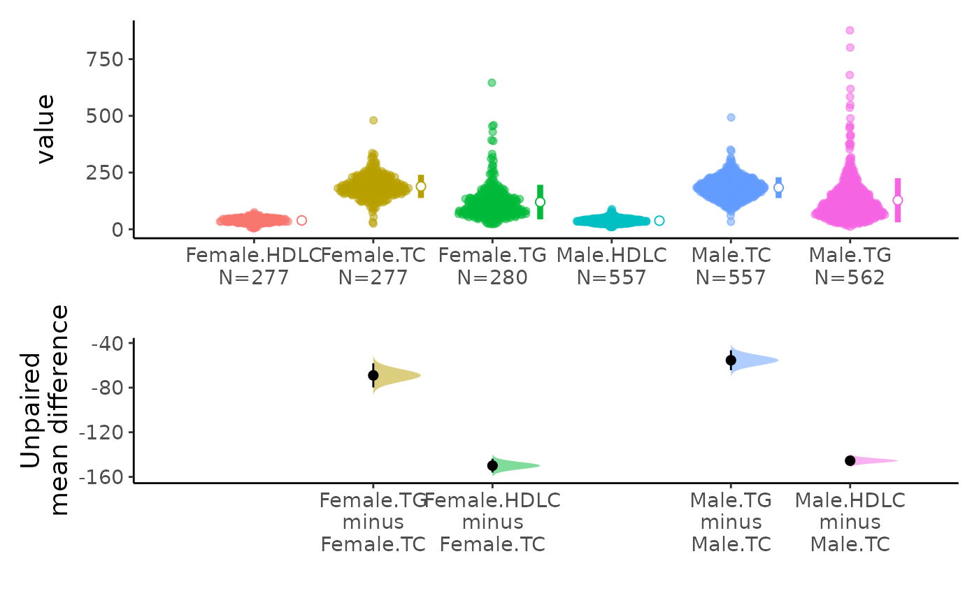 acs %>% select(sex,TC,TG,HDLC) %>% meanCI(sex) %>% plot()
#> Warning: Removed 61 rows containing missing values (position_quasirandom).
#> Warning: Removed 61 rows containing missing values (position_quasirandom).
#> Warning: Removed 61 rows containing missing values (position_quasirandom).
#> Warning: Removed 61 rows containing missing values (position_quasirandom).
acs %>% select(sex,TC,TG,HDLC) %>% meanCI(sex) %>% plot()
#> Warning: Removed 61 rows containing missing values (position_quasirandom).
#> Warning: Removed 61 rows containing missing values (position_quasirandom).
#> Warning: Removed 61 rows containing missing values (position_quasirandom).
#> Warning: Removed 61 rows containing missing values (position_quasirandom).
 # }
# }